Can I export a year’s worth of temperature data to Excel with a single click for charting?
In Fiber Bragg Grating (FBG) sensing and monitoring systems, ‘Historical Data Export’ typically refers to the process where the host computer software or system platform retrieves, extracts, and converts timestamp, channel number, wavelength value, temperature/strain engineering physical quantities, etc., stored in a local database (such as SQLite, MySQL, PostgreSQL, or time-series databases) according to specified conditions into external universal formats (e.g., CSV, TXT, XLSX, DAT, etc.).
Regarding your question – ‘Can I export a year’s worth of temperature data to Excel with one click for plotting?’ – from the perspective of engineering data computation and software limitations, it entirely depends on your data recording frequency (sampling interval). Directly exporting the full dataset is often limited by the physical constraints of Excel software’s underlying capacity.
I. Excel’s Hard Specification Limits
Microsoft Excel (standard .xlsx format from version 2007 onwards) has strict row and column limits for a single worksheet:
- Maximum Rows: 1,048,576 rows (i.e., 2^{20} rows)
- Maximum Columns: 16,384 columns
II. One Year Data Volume Calculation and Feasibility Analysis
A normal year has 365 days, with a total number of seconds:
365 \times 24 \times 3600 = 31,536,000 \text{ seconds}
1. High-Frequency Raw Sampling (Cannot be Directly Handled by Excel)
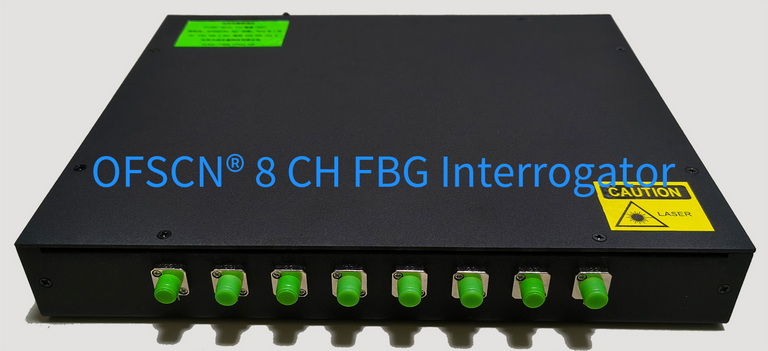
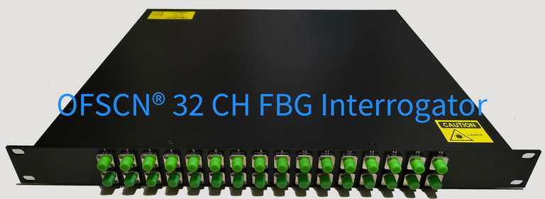
Fiber Bragg Grating interrogators usually have high sampling frequencies. For example, the OFSCN® Fiber Bragg Grating Interrogator typically has sampling frequencies of 10\text{ Hz}, 50\text{ Hz}, 100\text{ Hz}, which can be reduced to a minimum of 1\text{ Hz} through software downsampling:
- If stored at 1\text{ Hz} (i.e., 1 record per second): One year produces 31,536,000 records per measurement point.
- If stored at 10\text{ Hz}: One year produces 315,360,000 records per measurement point.
Conclusion: Even recording at a mere 1\text{ Hz}, the data volume already exceeds Excel’s single-sheet row limit (approx. 1.05 million rows) by 30 times. If you forcibly export directly to a single Excel file, Excel will not be able to load it completely, and it will result in truncation or software freezing and crashing.
2. Engineering Downsampling or Fixed-Point Storage (Completely Feasible)
In long-term static temperature monitoring projects, temperature is a slowly changing physical quantity, usually not requiring second-level or even sub-second storage density:
- Recording once every minute: The annual data volume is 365 \times 24 \times 60 = 525,600 records. This data volume is less than 1,048,576 rows, allowing it to be opened in a single Excel sheet and plotted directly as a line graph.
- Recording once every 10 minutes or 1 hour: The annual data volumes are 52,560 and 8,760 records, respectively, which are very lightweight and smooth to handle in Excel.
III. Typical Engineering Solutions for Historical Data Export
If you need to analyze and plot temperature monitoring data spanning a full year, it is recommended to adopt one of the following three engineering approaches:
- Downsampling during Export (Resampling / Downsampling):
In the system’s historical data query interface, set the export time step (e.g., export average, extreme, or instantaneous values every 5 minutes, 10 minutes, or 1 hour) to compress the total number of rows to within 1 million, enabling one-click export to Excel for plotting. - Export in Segments (Segmentation):
If high-density recording points must be retained (e.g., one record every few seconds), you can split the one-year time span into multiple CSV files exported by ‘month’ or ‘week’ and perform statistical analysis on each subset. - Utilize Professional Scientific Computing and Time-Series Analysis Tools:
If you must analyze and plot millions to hundreds of millions of raw second-level data points over a full year, it is recommended to export the historical data directly in standard CSV, TXT, or HDF5 formats, or query directly from the database, and then use professional tools for processing:- Python (using Pandas / Polars for table manipulation, Matplotlib / Seaborn for plotting)
- MATLAB / OriginPro
These tools are specifically designed for memory optimization and GPU plotting pipelines, capable of stably handling massive datasets with tens of millions of rows.
IV. Associated Equipment and Software Architecture
The OFSCN® Fiber Bragg Grating Interrogator adopts a B/S or C/S software architecture by default, with the following core parameters:
- Data Sampling Frequency: Supports 10\text{ Hz}, 50\text{ Hz}, 100\text{ Hz} (users can independently reduce the sampling frequency via software, with a minimum support of 1\text{ Hz}).
- Wavelength and Channels: Covers 4, 8, 16, 32 channels, with wavelength resolution of 1\text{ pm} or 0.1\text{ pm}.
- System Integration and Dumping: Supports standard protocols such as TCP, UDP, and Modbus, facilitating the docking of real-time and historical data streams to industrial host systems or third-party databases for long-term storage and secondary processing.