Why use mathematical formulas to fit the reflection peak? Can it improve accuracy?
In Fiber Bragg Grating (FBG) sensing technology, using mathematical formulas such as Gaussian fitting to fit the reflection spectrum peak is not only necessary but also a core method for significantly enhancing the measurement accuracy and resolution of demodulation systems.
The underlying physical and engineering reasons can be academically analyzed from the following three perspectives:
1. Conflict Between the “Continuity” of Physical Reflection Spectrum and the “Discreteness” of Hardware Sampling
Physically, a Fiber Bragg Grating (FBG) reflects a continuous spectrum, with its theoretical reflectivity distribution closely resembling Gaussian, Lorentzian, or Sinc functions.
However, in actual measurements, FBG demodulators (whether they are spectrometer-based using CCD/InGaAs linear array detectors or scanning-based using tunable lasers) perform discrete sampling of this reflection peak. The pixels on the photosensitive chip or the wavelength steps of the laser cut the continuous spectrum into a finite number of discrete data points.
-
Limitations of the “Direct Peak Finding Method” (Finding the Maximum Value):
If a mathematical formula is not used for fitting, and the point with the highest light intensity among the discrete sampling points is directly identified as the center wavelength of reflection, then the measured wavelength resolution will be entirely limited by the hardware physical sampling interval (pixel resolution) of the demodulator.For example, if the physical sampling interval of the demodulator is 40\text{ pm} , without using mathematical fitting, the system’s ultimate wavelength resolution would only be 40\text{ pm} . In practical sensing, a drift of 40\text{ pm} typically corresponds to a temperature change of about 4\text{ }^\circ\text{C} or a strain of 40\ \mu\varepsilon . Such coarse resolution is unusable in high-precision industrial and scientific measurements.
2. How Mathematical Fitting Achieves “Sub-pixel” Super-resolution?
The Gaussian Fitting Method overcomes the physical limitations of the hardware’s physical sampling interval by incorporating the discrete experimental data points into a known Gaussian mathematical model.
The general mathematical expression for a Gaussian reflection peak is:
I(\lambda) = I_0 \exp\left( -4 \ln 2 \frac{(\lambda - \lambda_B)^2}{\Delta \lambda^2} \right)
Where:
- I(\lambda) is the reflected light intensity at wavelength \lambda ;
- \lambda_B is the Bragg center wavelength we need to find;
- \Delta \lambda is the 3\text{ dB} bandwidth of the reflection peak.
After acquiring several discrete data points near the reflection peak (typically using points where the reflectivity is in the range of -3\text{ dB} to -10\text{ dB} ), the demodulator uses logarithmic linear fitting or least squares nonlinear regression algorithms to inversely solve for the theoretical symmetrical center axis \lambda_B of the Gaussian curve.
Through this mathematical interpolation and regression calculation, the output value of the center wavelength \lambda_B is no longer limited by the position of the pixels but becomes a high-precision continuous floating-point number. This can directly improve the wavelength resolution from the physical sampling interval (e.g., 40\text{ pm} ) to 1\text{ pm} or even 0.1\text{ pm} . The accuracy and resolution are thus improved by 100 to 400 times.
3. Suppressing Random Noise and Improving Measurement Stability
During the actual optoelectronic signal conversion and transmission process, the signal inevitably accumulates spontaneous emission (ASE) noise from the light source, detector thermal noise, and dark current noise.
- If a simple “find the maximum point” method is used, any slight jitter in a sampling point near the maximum value due to noise will cause the demodulated wavelength value to jump, resulting in a large measurement standard deviation.
- The Gaussian fitting algorithm, however, utilizes a set of data points on the reflection spectrum for overall fitting. In mathematical regressions like the method of least squares, random noise from individual sampling points is averaged and diluted during the summation calculation. This statistical averaging effect on noise gives the fitting algorithm strong noise immunity, thereby making the demodulated wavelength highly repeatable and stable.
Application in Practical Systems
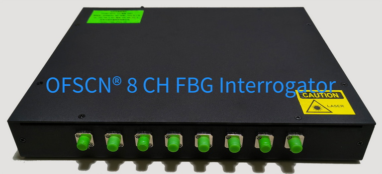
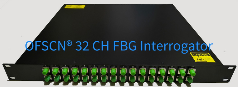
In precision fiber optic sensing applications, excellent demodulator firmware and host computer software integrate such algorithms. For instance, when the OFSCN® Fiber Bragg Grating Interrogator processes spectral data from FBGs, it uses its built-in high-performance fitting and peak-finding algorithms to stably provide an ultra-high wavelength resolution of the default 1\text{ pm} , or even a customizable 0.1\text{ pm} , despite limited sampling hardware.
This sub-picometer (Sub-pm) level wavelength resolution provided by these algorithms is the technical cornerstone that enables products such as the OFSCN® 300°C Fiber Bragg Grating Temperature Sensor or various OFSCN® FBG Strain Sensor Products Aggregation to output high-resolution, high-repeatability physical quantity data.